Commonly in neuroscience research, animal brains are probed with electrodes, measuring voltage signals from neurons while the animal performs a task. Electrodes have become so advanced nowadays that they can contain hundreds of sensors on a probe about the size of a human hair. During data analysis, this high dimensionality creates problems in computation and interpretation. It is hard to see what a 100-dimensional object looks like. Because of this, there has been a push towards dimensionality reduction models in neuroscience research. Researchers can reduce the 100 neurons down to 2 dimensions, allowing them to be visualized on a graph. Given that the data is recorded over time, the researchers can observe how the neurons "move" in this 2-D space. When these variables are plotted, they can be interpreted as neural trajectories.
The premise behind these models is that although the brain may be complex, maybe the underlying phenomenon is simple. For example, when you walk there are many millions of neurons firing, yet walking is simple, and so maybe the behavior of the millions neurons can be explained with just a few variables. For terminology, dimensionality reduced variables will be called latent variables, because they are not observed, but explain the observed data.
For our project, we use Latent Variable Models to extract neural trajectories from a mouse as it performs a decision-making task.
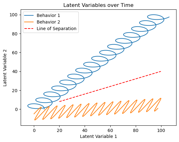
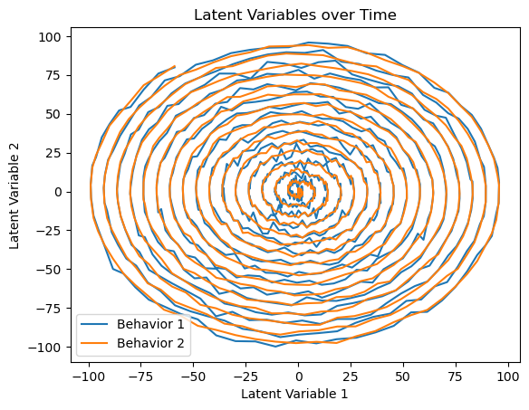
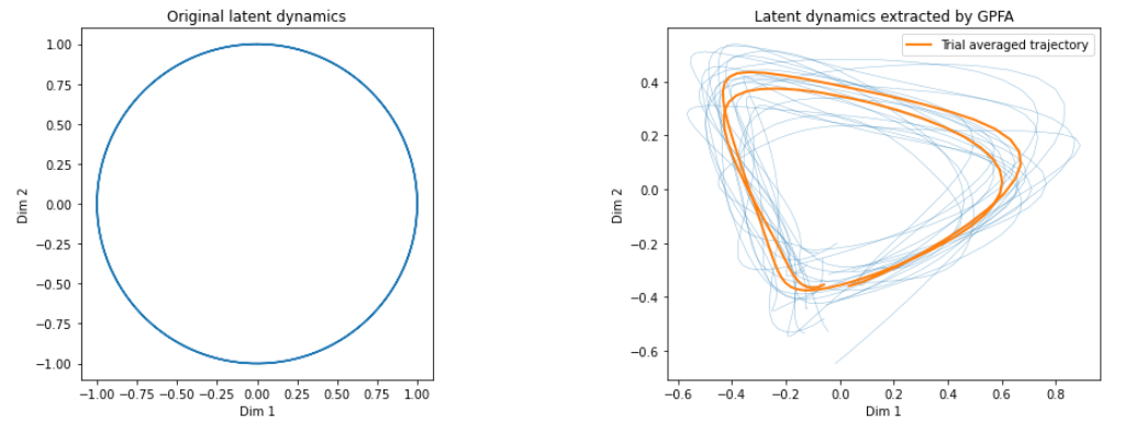
We are trying to predict whether a mouse will turn a wheel clockwise (Wheel Turned Right) or counter-clockwise (Wheel Turned Left). By plotting our neural trajectories, we may observe that there is a difference in the brain's "path" when the mouse turns a wheel clockwise vs counter-clockwise. We will use this difference to create a classification algorithm to predict which direction the mouse will choose. Figures 1 and 2 show example trajectories that we might obtain.
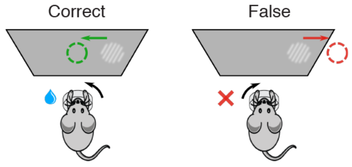
We use data collected by the International Brain Laboratory [IBL], which inserted Neuropixel probes into mice brains as they performed a decision making task. The task was as follows:
The mouse repeated this task hundreds of times with probes inserted in its brain recording voltage signals at 384 locations. IBL has taken this raw electrophyisology data and performed their own preprocessing to give us neuronal units (clusters) and their spike times.
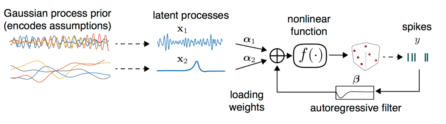
Gaussian Process Factor Analysis (GPFA) models the observed data, y, as a linear combination of low-dimensional latent variables, z, using a Gaussian process. The latent variables are modeled as a Gaussian process with mean, m, and covariance function, k_z(z_i, z_j). The observed data is modeled as a linear combination of the latent variables, given by y = Cz + ε, where C is a loading matrix and ε is a noise term.
The goal of GPFA is to infer the latent variables and the loading matrix given the observed data. This can be done using maximum likelihood estimation by maximizing the log-likelihood of the data, given by:
where K_y = CC^T + σ^2I is the covariance matrix of the observed data and σ^2 is the noise variance. The solution provides estimates of the latent variables and the loading matrix, which can be used to reconstruct the underlying patterns in the data.
Variational Latent Gaussian Process (VLGP) extends the standard Gaussian Process (GP) by introducing a latent variable model to capture the underlying dynamics of the time series. The latent variables z are modeled as a Gaussian Process with mean function m(z_t) and covariance function k(z_t, z_t').
VLGP uses variational inference to learn the latent trajectories and basis functions by optimizing the Evidence Lower Bound (ELBO), given by:

where q(z_{1:T}) is an approximate posterior distribution over the latent variables, and p(z_{1:T}) is the prior distribution over the latent variables defined by the GP. The first term of the ELBO encourages the model to generate data that is consistent with the observed data, while the second term encourages the approximate posterior distribution to be close to the prior distribution. Using the posterior distribution, we can capture the underlying dynamics of our neural data.
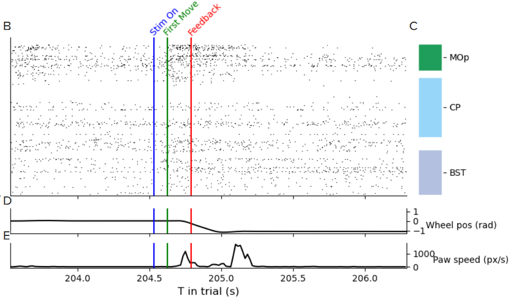
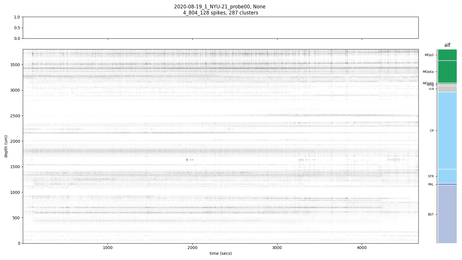
From Figure 7, we can see a flurry of neural activity in the MOp as the mouse begins to move. This increase in firing rate is what we hope to capture in our model.
We chose to analyze data that came from the Primary Motor Cortex (MOp). We believed that the trajectories obtained from this region would be more differentiable between the different behaviors we expect the mouse to engage in.
Furthermore, we filtered clusters based on their quality. IBL has a metric for determining how "good" a cluster is, which indicates their confidence that the spikes came from a single unit. A bad cluster would indicate that IBL thinks the spike could have come from multiple units, which could add noise to our data.
We train the model on a window that begins 0.1 seconds before the mouse starts moving to 1 second after the mouse started moving. This should allow us to see how the brain changes throughout the mouse's actions.
Shown below are trajectories we obtained using a variety of methods.
From Figure 8 we can see that the trajectories start off very different, but then begin to blend together as time goes on. This indicates that very specific processes are occurring in the brain early after the mouse begins moving the wheel. Figure 10 shows 3 latent variables, and it might be possible to say the trajectries are separable, however without a time dimension it is difficult to tell when this separability occured.
As mentioned before, we want to see a clean separation between the trial types which we can observe in Figure 8 at Time=100ms. Using this information, we take a slice of the data at Time=100ms.
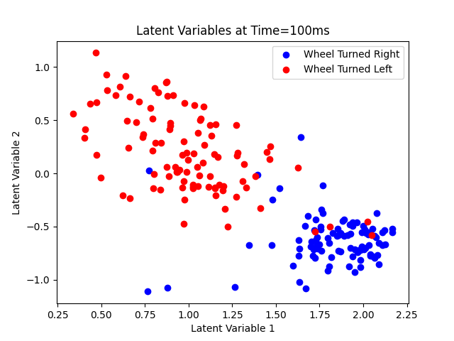
Figure 11 shows very discernable classes which we train a Logistic Regression Classifier on.
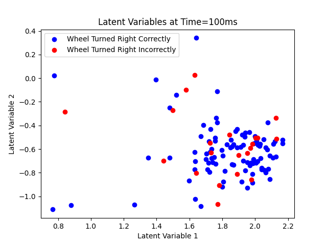
Figure 12 shows very poor separation between the classes, but we train a Logistic Regression Classifier on it to see how well it can perform.
Due to an imbalanced test set, we use the metric Balanced Accuracy to evaluate our classifiers. The higher the balanced accuracy, the better the classifier performed. We evaluated the classifiers in 3 different scenarios, using no dimensionality reduction vs using 2 latent variables, using vLGP vs GPFA, and predicting between Class 0 or Class 1 and Class 0 or Class 2.
Class 0 is when the mouse correctly moved the wheel clockwise, Class 1 is when the mouse correctly moved the wheel counter-clockwise, Class 2 is when the mouse incorrectly moved the wheel clockwise, and Class 3 is when the mouse incorrectly moved the wheel counter-clockwise however it is not used in this analysis.
| # of Latent Variables | Method of Dimensionality Reduction | Classes | Balanced Accuracy |
|---|---|---|---|
| N/A | No Dimensionality Reduction | Class 0 vs Class 1 | 94% |
| 2 | vLGP | Class 0 vs Class 1 | 93% |
| 2 | GPFA | Class 0 vs Class 1 | 91% |
| 2 | vLGP | Class 0 vs Class 2 | 50% |
| 2 | GPFA | Class 0 vs Class 2 | 50% |
As can be seen from the table above, the classifier that did not use dimensionality reduction performed the best. This contrary from what we were expecting, which was to see better classification using latent variable models. We also see that vLGP outperforms GPFA, which is what we expect since vLGP is able to extract more accurate latent variables. Both latent variable models perform poorly when trying to discern whether the mouse turned the wheel clockwise correctly or incorrectly.
We observe that our latent variable models performed more poorly compared to using no dimensionality reduction. This is most likely due to the loss of information that occurs when reducing dimensionality, however it is possible when analyzing a larger number of neurons that the accuracy would suffer due to noise. In general GPFA and vLGP are able to filter out noise and so might overtake the performance non-dimensionality reduced classifiers at very high dimensionality. There is still value in using latent variable models in this instance as it allowed us to visualize how the brain "moved" over time. As we saw in Figure 8, there was clear separation in the motor cortex around 100ms, but then the latents became seemingly random, showing that the mouse's movement will cause separation, and once the mouse stops moving the activity in the brain becomes random again.
Being able to discern behaviors using the neural signals indicate that there are distinct processes in the motor cortex when the mouse turns the wheel clockwise vs counter-clockwise. This makes sense as we would expect different neurons to fire when controlling different muscles. On the other hand, we see no difference in the brain when the mouse turns the wheel clockwise correctly vs incorrectly. This makes sense since we are analyzing the motor cortex, and the actions taken during these 2 behaviors are the same. It is mostly likely difficult to find separation between correct vs incorrect, since the mouse believes what it is doing to be correct, otherwise it would not have made a mistake.
The results we got were from a lot of trial and error in choosing brain regions, bin sizes, and mice. In another mouse following the same procedure, we obtained no separability in the trajectories even though we analyzed the same brain region (Primary Motor Cortex). This indicates that different parts of the primary motor cortex are responsible for different muscles, and you have to carefully select brain regions which shows a change in activity in response to the task.